Stats with R - 4

Salary can be influenced by many variables. Among these, years of professional experience and total courses completed in college are critical.  we test this hypothesis with a simulated dataset including an outcome variable, salary, and two predictors, years of experience and courses completed. Here are a few questions based on what was covered in the lectures and the lab. Have fun!

 Source DataSet :-   https://spark-public.s3.amazonaws.com/stats1/datafiles/Stats1.13.HW.04.txt

Glimpse of the Dataset :-

To read in the Data set :-
PE<- read.table("Stats1.13.HW.04.txt",header = T)

1.What is the correlation between salary and years of professional experience?

R- code
> round(cor(PE$salary ,PE$years),2)
[1] 0.74

2.What is the correlation between salary and courses completed?

R- code
> round(cor(PE$salary , PE$courses),2)
[1] 0.54

3.What is the percentage of variance explained in a regression model with salary as the outcome variable and professional experience as the predictor variable?
Ans : 55 

R- code
model1<- lm(PE$salary ~ PE$years)
summary(model1)

4 .Compared to the model from Question 3, would a regression model predicting salary from the number of courses be considered a better fit to the data?
we need to compare here model1 and model4

R- code
model1<- lm(PE$salary ~ PE$years)
summary(model1)

model4 <- lm(PE$salary ~ PE$courses)

summary(model4)

Since the re-gression co-efficient  is  higher in model1 , MODEL1 regression model with salary as the outcome variable and professional experience as the predictor variable will be a better fit than  MODEL4
predicting salary from the number of courses be considered a better fit to the data .

5. Now let's include both predictors (years of professional experience and courses completed) in a regression model with salary as the outcome. Now what is the percentage of variance explained?
Ans :- 65 

R- code
model2<- lm(PE$salary ~ PE$years+PE$courses)

summary(model2)

6 .What is the standardized regression coefficient for years of professional experience, predicting salary?
Ans :- .74
R- code
model6 <- lm(scale(PE$salary) ~ scale(PE$years))
summary(model6)

7.What is the standardized regression coefficient for courses completed, predicting salary?
Ans:- .54
R- code
model7<- lm(scale(PE$salary) ~ scale(PE$courses))
summary(model7)

8.What is the mean of the salary distribution predicted by the model including both years of professional experience and courses completed as predictors? (with 0 decimal places)
Ans :- 75426
R- code
model2<- lm(PE$salary ~ PE$years+PE$courses)
summary(model2)
> PE$predicted <- fitted(model2)
> mean (PE$predicted)
[1] 75426.44

9.What is the mean of the residual distribution for the model predicting salary from both years of professional experience and courses completed? (with 0 decimal places)
Ans :-  0
R- code
model2<- lm(PE$salary ~ PE$years+PE$courses)
summary(model2)
> PE$residual <- resid(model2)
> mean(PE$residual)
[1] -1.893208e-14

10 .Are the residuals from the regression model with both predictors normally distributed?
Ans :- YES
 R- code
model2<- lm(PE$salary ~ PE$years+PE$courses)
summary(model2)
PE$residual <- resid(model2)

hist(PE$residual)

Stats with R - 3

Case study :-  Cognitive training is a rapidly growing market with potential to further expand in the future. Several computerized software programs promoting cognitive improvements have been developed in recent years, with controversial results and implications. In a distinct literature, aerobic exercise has been shown to broadly enhance cognitive functions, in humans and animals. My research group is attempting to bring together these two trends of research, leading to an emerging third approach: designed sport training. Specifically designed sports are an optimal way to combine the benefits of traditional cognitive training and aerobic exercise into a single activity. So, suppose we conducted a training experiment in which subjects were randomly assigned to one of two conditions: Designed sport training (des)
 and Aerobic training (aer). Also, assume that we measured both verbal and spatial reasoning before and after training, using four separate measures: • S1 • S2 • V1 • V2. Simulated data are available here. Save the file to your computer and read it into R to complete the assignment and answer the following questions.

Source DataSet :- https://spark- public.s3.amazonaws.com/stats1/datafiles/Stats1.13.HW.03.txt

The data set somewhat  looks like this :-

                                                                               



Reading in the dataset in R   
data <- read.table("Stats1.13.HW.03.txt",header = T)

1.What is the correlation between S1 and S2 pre-training?
Ans:- 0.49 (rounding to two significant digit )
R- code 
> cor(data$S1.pre, data$S2.pre)
[1] 0.4920231

2.What is the correlation between V1 and V2 pre-training?
Ans:- 0.90 (rounding to two significant digit )
R- code 
> cor(data$V1.pre, data$V2.pre)
[1] 0.9038863

3. With respect to the measurement of two distinct constructs, spatial reasoning and verbal reasoning, the pattern of correlations pre-training reveals:
Ans :- The pattern of correlations pre- training reveals BOTH Convergent validity and  Divergent validity

R- code 
> data$V.pre = (data$V1.pre + data$V2.pre)/ 2
> data$S.pre = (data$S1.pre + data$S2.pre)/ 2
> cor(data$S.pre, data$V.pre)
[1] 0.1186354

4.Correlations from the control group could be used to estimate test/retest reliability. If so, which test is most reliable? ---
 Ans :- V2

R- code 
> data.aer = subset(data, data$cond=="aer")
> cor(data.aer$S1.pre, data.aer$S1.post)
[1] 0.6277946
> cor(data.aer$S2.pre, data.aer$S2.post)
[1] 0.633611
> cor(data.aer$S1.pre, data.aer$S1.post)
[1] 0.6277946
> cor(data.aer$S2.pre, data.aer$S2.post) 
[1] 0.633611
> cor(data.aer$V1.pre, data.aer$V1.post)
[1] 0.744725
> cor(data.aer$V2.pre, data.aer$V2.post)  - #This test is more reliable
[1] 0.9075993

5 .Does there appear to be a correlation between spatial reasoning before training and the amount of improvement in spatial reasoning?
Ans :- No 
(This is because the variables spatial reasoning (data$S.pre) and  amount of improvement in spatial reasoning (data$Sgain) are negatively correlated
R- code 
> data$S.pre = (data$S1.pre + data$S2.pre) / 2
> data$S.post = (data$S1.post + data$S2.post) / 2 
> data$Sgain = data$S.post - data$S.pre 
> cor(data$S.pre, data$Sgain)
[1] -0.09280867

6 .Does there appear to be a correlation between verbal reasoning before training and the amount of improvement in verbal reasoning? 
Ans :- No 
(This is because the variables  verbal reasoning (data$V.pre) and  improvement in verbal reasoning (data$Vgain) are negatively correlated
R- code 
> data$V.pre = (data$V1.pre + data$V2.pre)/ 2
> data$V.post = (data$V1.post + data$V2.post) / 2
> data$Vgain = data$V.post - data$V.pre
> cor(data$V.pre, data$Vgain)

[1] -0.05822132

7.Which group exhibited more improvement in spatial reasoning?
Ans :- des 

R- code 

8. Create a color scatterplot matrix for all 4 measures at pre-test. Do the scatterplots suggest two reliable and valid constructs? 
Ans :- YES
R- code 
base <- cbind(data[3], data[4], data[7], data[8])
base.r <- abs(cor(base))
base.color <- dmat.color(base.r)
base.order <- order.single(base.r)
cpairs(base,base.order ,panel.color = base.color,gap = .5,main = "Variables ordered and colored by correlation")

9 Create a color scatterplot matrix for all 4 measures at post-test. Do the scatterplots suggest two reliable and valid constructs?
Ans :- YES
R- code 
base <- cbind(data[5], data[6], data[9], data[10])
base.r <- abs(cor(base))
base.color <- dmat.color(base.r)
base.order <- order.single(base.r)
cpairs(base,base.order ,panel.color = base.color,gap = .5,main = "Variables ordered and colored by correlation")

                                                                                                                                           

 10 What is the major change from pre-test to post-test visible on the color matrix?
  Ans : Variance

Stats with R - 1

Source DataSet :- https://spark-public.s3.amazonaws.com/stats1/datafiles/Stats1.13.HW.02.txt

Initially I read the text file in form of a dataframe in R by running the following command ,I named the dataframe as "impact" :-

> impact <- read.table("Stats1.13.HW.02.txt",header = T)

A data set with 96 obsetvations and 4 varibles is created in R

1.How many rows of data are in the data file?
96
Make sure you read the data with the argument: header=TRUE Then: nrow(data) OR dim(data)

2.What is the name of the dependent variable?
command : names(data)
Ans : SR 

3.What is the mean of SR across all subjects? 
command : mean(data$SR) OR describe(data)

> mean(impact$SR)
[1] 12.65625


4.What is the variance of SR across all subjects?
Command : var(data$SR

output :
> var(impact$SR)
[1] 6.54375

5.What is the mean of SR for all subjects at pretest?
command :- pre = subset(data, data$time=="pre") THEN mean(pre$SR)

Output :
> pre<- subset(impact,impact[ ,3]== "pre")
> mean(pre$SR)
[1] 12.02083

6.What is the standard deviation of SR for all subjects at posttest?
command :- post = subset(data, data$time=="post") THEN sd(post$SR)

Output :
> sd(post$SR)
[1] 2.449128

7.What is the median of SR for all subjects at posttest?
describe(post$SR) AND median(post$SR)

Output:-
> describe(post$SR) 
  var  n  mean   sd  median trimmed  mad min max range skew kurtosis   se
1   1 48 13.29  2.45   13.5   13.28     2.22   9  19    10     0.06    -0.49    0.35
> median(post$SR)
[1] 13.5

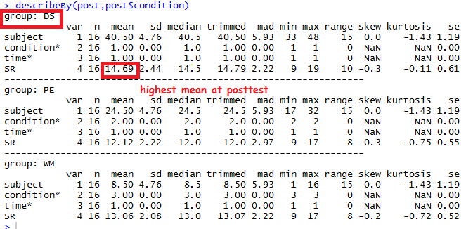
8.Which group has the highest mean at posttest?
Ans :- DS
.Command :- describeBy(post, post$condition)

Output :-

9.Which one best approximates a normal distribution?
 Option :- 

WM group at pretest
WM group at postest    Ans :- WM group at postest	Correct
PE group at pretest
PE group at posttest
DS group at pretest
DS group at postest Code :-

pre.wm = subset(pre, pre$condition=="WM")
post.wm = subset(post, post$condition=="WM")
pre.pe = subset(pre, pre$condition=="PE")
post.pe = subset(post, post$condition=="PE")
pre.ds = subset(pre, pre$condition=="DS")
post.ds = subset(post, post$condition=="DS")
par(mfrow= c(2,3))
hist(pre.wm[,4])
hist(post.wm[,4])
hist(pre.pe[,4])
hist(post.pe[,4])
hist(pre.ds[,4])
hist(post.ds[,4])

10.Which group showed the biggest gains in SR?
Code :-
pre.wm = subset(pre, pre$condition=="WM")
post.wm = subset(post, post$condition=="WM")
pre.pe = subset(pre, pre$condition=="PE")
post.pe = subset(post, post$condition=="PE")
pre.ds = subset(pre, pre$condition=="DS")
post.ds = subset(post, post$condition=="DS")
> mean(post.wm$SR)-mean(pre.wm$SR) 
[1] 1.3125
> mean(post.pe$SR)-mean(pre.pe$SR) 
[1] 0.0625
> mean(post.ds$SR)-mean(pre.ds$SR)
[1] 2.4375

ANS :- DS

Basics of R

The two packages in R required for descriptive Statistics :
First we need to install  the following packages and then load them in R
install.packages("psych")
install.packages("sm")

Reading a text file in R:
Text <- read.table("file.txt",header = T)
Make sure you read the data with the argument: header=TRUE .R does not read the 1st line and continues reading from the second line

Command to find no of rows in  a data file :
nrow(data) OR dim(data)

Output :-
> dim(Text)
[1] 96  4

> nrow(Text)
[1] 96

Subsetting a dataset :

Command :-
New <- subset(impact,impact[ ,3]== "updated")

Here we are subsetting on the variables of the 3rd column  into New dataset  . we are only selecting the variables og the 3rd column which has an  value "post"


To obtain a descriptive statistic of a dataset :
Suppose we have a dataset named "impact". The describe function gives us the  all possible statistic of all variable of that dataset

what is the utility of  describeBy function in R ?
DescribeBy function gives you the summary statistic by categorical variable of a defined column