Friday, December 6, 2013
Sunday, December 1, 2013
Stats with R - 8 (Logistic Regression)
This week we are going to work on an example at the intersection of decision-making and global warming. The simulated dataset includes a dependent variable, change, for a list of 27 countries. Change indicates whether these countries are willing to take action now against global warming, or if they would rather wait and see (1 = act now, 0 = wait and see). Predictors include: median age (age), education index (educ), gross domestic product (gdp), and CO2 emissions (co2).
BL <- read.table("stats1-datafiles-Stats1.13.HW.10.txt",header= T)
Glimpse of the Dataset :-

1.What is the median population age for the countries which voted to take action against global warming? (round to 2 decimal places)
Ans:- 35.78
R- Output

2.Run a logistic regression including all predictor variables. Which predictors are significant in this model?
ANS :-The predictors educ and age are significant with a p value lower than .05
lrfit = glm(BL$change ~ BL$educ + BL$age + BL$gdp + BL$co2, family = binomial)
summary(lrfit)
R- Output

3. What does the negative value for the estimate of educ means?
4 .What is the confidence interval for educ, using profiled log-likelihood? (round to 2 decimal places, and give the lower bound first and the upper bound second, separated by a space)
Ans :- -31.17 -3.03
confint(lrfit)
R- Output
> confint(lrfit)
2.5 % 97.5 %
(Intercept) -7.120294915 7.62212837
BL$educ -31.171217249 -3.03349629
BL$age 0.151757331 0.73814438
BL$gdp -1.677996402 0.67880052
BL$co2 -0.001889047 0.00185111
5 . What is the confidence interval for age, using standard errors? (round to 2 decimal places, and give the lower bound first and the upper bound second, separated by a space)
Ans :- 0.09 0.65
R- Output
confint.default(lrfit)
2.5 % 97.5 %
(Intercept) -7.016319882 6.981360625
BL$educ -27.332984665 -0.119112070
BL$age 0.092877885 0.651260815
BL$gdp -0.986127869 0.835048069
BL$co2 -0.001910404 0.001148391
6. Compare the present model with a null model. What is the difference in deviance for the two models? (round to 2 decimal places)
Ans :- 16.30
R- Output
> with(lrfit, null.deviance - deviance)
[1] 16.30328
7. How many degrees of freedom are there for the difference between the two models?
Ans:- 4
R- Output
> with(lrfit, df.null - df.residual)
[1] 4
8.Is the p-value for the difference between the two models significant?
Ans:- Yes
R- Output
> with(lrfit, pchisq(null.deviance-deviance, df.null-df.residual, lower.tail = FALSE))
[1] 0.002638074 ---- this indicates that it is significant
9.Do chi-squared values differ significantly if you drop educ as a predictor in the model?
Ans :- Yes
R- Output
> wald.test(b = coef(lrfit), Sigma = vcov(lrfit), Terms = 2)
Wald test:
----------
Chi-squared test:
X2 = 3.9, df = 1, P(> X2) = 0.048
10. What is the percentage of cases that can be classified correctly based on our model?
Ans:- 81
R- Output
> ClassLog(lrfit, BL$change)
$rawtab
resp
0 1
FALSE 6 2
TRUE 3 16
$classtab
resp
0 1
FALSE 0.6666667 0.1111111
TRUE 0.3333333 0.8888889
$overall
[1] 0.8148148
Wednesday, November 27, 2013
Stats with R - 7
Source DataSet :- https://d396qusza40orc.cloudfront.net/stats1%2Fdatafiles%2FStats1.13.HW.07.txt
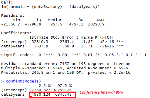
Run a regression model with salary as the outcome variable and years of experience as the predictor variable. What is the 95% confidence interval for the regression coefficient? Type your answer exactly as it appears in R but include only two decimal places (for example, if the 95% confidence interval is -1 to +1 then type -1.00 1.00)
Ans :- 27360.82 38259.76
Question Explanationmodel1 = lm(data$salary ~ data$years) AND confint(model1)
Run a regression model with salary as the outcome variable and courses as the predictor variable. What is the 95% confidence interval for the regression coefficient?
Ans:- 59656.54 65782.32
Question Explanationmodel2 = lm(data$salary ~ data$courses) AND confint(model2)
3 .Run a multiple regression model with both predictors and compare it with both the model from Question 1 and the model from Question 2. Is the model with both predictors significantly better than:
both single predictor models
the single predictor model based on years of experience
the single predictor model based on courses
none of the above
Question Explanationmodel3 = lm(data$salary ~ data$years + data$courses) AND anova(model1, model3) AND anova(model2, model3)
Run a standardized multiple regression model with both predictors. Do the confidence interval values differ from the corresponding unstandardized model?
Ans :- yes
model3.z = lm(scale(data$salary) ~ scale(data$years) + scale(data$courses)) AND confint(model3.z)
What function could you use to take a random subset of the data?
sample
Run the following command in R: set.seed(1). Now take a random subset of the original data so that N=15. Is the correlation coefficient between salary and years of experience in this sample higher or lower than in the whole data set?
Ans :- Lower
Wednesday, November 13, 2013
Stats with R - 6
data<- read.table("Stats1.13.HW.04.txt",header = T)
In a model predicting salary, what is the unstandardized regression coefficient for years, assuming years is the only predictor variable in the model?
5638
data <-read.table("week6.txt",header = T)summary(model1 <- lm((data$salary) ~ (data$years)))
In a model predicting salary, what is the 95% confidence interval for the unstandardized regression coefficient for years, assuming years is the only predictor variable in the model?
4930 6345
data <-read.table("week6.txt",header = T)
summary(model1 <- lm((data$salary) ~ (data$years)))
confint(model1)
In a model predicting salary, what is the unstandardized regression coefficient for years, assuming years and courses are both included as predictor variables in the model?
4807
summary(model2 <- lm((data$salary) ~ (data$years)+(data$courses)))
In a model predicting salary, what is the 95% confidence interval for the unstandardized regression coefficient for years, assuming years and courses are both included as predictor variables in the model?
4140 5473
summary(model2 <- lm((data$salary) ~ (data$years)+(data$courses)))
confint(model2)
What is the predicted difference in salary between Doctors and Lawyers assuming an equal and average number of years and courses?
9204
Sunday, November 10, 2013
Stats with R - 5
1.Which of the following are characteristics of experimental research?
a .Random sampling from a population
b. Random assignment to treatment conditions
Both a and b
2.The distribution of household income in the United States, currently, is:
Positively skewed
3.When distributions are skewed, the most accurate measure of central tendency is:
The median
4.Given a distribution of scores, the average of the squared deviation scores is equal to:
The variance
5.Complete the following syllogism: SS is to SD as SP is to:
Correlation
6.Pearson’s product moment correlation coefficient (r) is used when X and Y are:
Both continuous variables
7.Which of the following pairs of variables is most likely to be negatively correlated?
Hours watching TV per week and college GPA
8.Systematic measurement error represents:
bias
9.We all know that correlation does not imply causation but correlations are useful because they can be used to assess:
Reliability,Validity,Prediction errors
10.In a regression analysis, which distribution will have the largest standard deviation?
the observed scores on the outcome variable, Y
11.The difference between an observed score and a predicted score in a regression analysis is known as:
Residual
12.In a simple regression analysis with outcome variable Y, the standardized regression coefficient for X will always equal:
The correlation coefficient
13.If the regression line in a scatterplot is horizontal then what is the regression coefficient?
0
14.In a regression analysis, if the residuals are correlated with X then what assumption has most likely been violated?
homoscedasticity assumption
15.When converting from an unstandardized to a standardized multiple regression analysis which of the following values will change?
regression coefficients
16.In multiple regression what is the difference between R and R^2?
R is the correlation between predicted and observed scores whereas R^2 is the percent of the variance in Y that can be explained by the regression model
17.In the faculty salary example, Ŷ = 46,910 + (1,382)X1 + (502)X2 – (3,484)X3, where X1 = years since graduation, X2 = publications, and X3 = gender (male coded as 0 and female coded as 1). According to this model, the predicted salary for a male faculty member who just graduated (years = 0), with zero publications, is:
Ans : $46,910
18.In the faculty salary example the actual difference in average salary between men and women was NOT = $3,484. $3,484 is:
The predicted difference between male and female faculty who are average in years since they graduated and have an average number of publications
19.In multiple regression analysis, the null hypothesis assumes that the unstandardized regression coefficient, B, is zero. The standard error of the regression coefficient depends on:
Sample size, Sum of Squared Residuals, and the number of other predictor variables in the regression model
20.When conducting a null hypothesis significance test, the p value represents:
The probability of the data given the null hypothesis is true

21.Use the R output above to answer the 5 questions below. The R output is from a quick analysis conducted on data collected at Columbia University and demonstrates a slight positive correlation between overall SAT score (sat) and proportion of items recalled on a working memory span task (span1). What is the unstandardized regression coefficient for working memory span in the regression equation predicting SAT?
300.9
22.R output. What is the predicted SAT score for a student who scored .50 on the working memory span task (round to a possible SAT score, for example, 2400 is a possible score, 2399.56 is not)?
2000
23.R output. What percentage of variance in SAT is explained by working memory span?
3
24.R output. What is the standard error of the sampling distribution of unstandardized regression coefficients?
211.2
Sunday, October 20, 2013
Stats with R - 4
Salary can be influenced by many variables. Among these, years of professional experience and total courses completed in college are critical. we test this hypothesis with a simulated dataset including an outcome variable, salary, and two predictors, years of experience and courses completed. Here are a few questions based on what was covered in the lectures and the lab. Have fun!
Source DataSet :- https://spark-public.s3.amazonaws.com/stats1/datafiles/Stats1.13.HW.04.txt
Glimpse of the Dataset :-

To read in the Data set :-
PE<- read.table("Stats1.13.HW.04.txt",header = T)
1.What is the correlation between salary and years of professional experience?
R- code
> round(cor(PE$salary ,PE$years),2)
[1] 0.74
2.What is the correlation between salary and courses completed?
R- code
> round(cor(PE$salary , PE$courses),2)
[1] 0.54
3.What is the percentage of variance explained in a regression model with salary as the outcome variable and professional experience as the predictor variable?
Ans : 55
R- code
model1<- lm(PE$salary ~ PE$years)
summary(model1)

4 .Compared to the model from Question 3, would a regression model predicting salary from the number of courses be considered a better fit to the data?
we need to compare here model1 and model4
R- code
model1<- lm(PE$salary ~ PE$years)
summary(model1)

model4 <- lm(PE$salary ~ PE$courses)
summary(model4)

Since the re-gression co-efficient is higher in model1 , MODEL1 regression model with salary as the outcome variable and professional experience as the predictor variable will be a better fit than MODEL4
predicting salary from the number of courses be considered a better fit to the data .
5. Now let's include both predictors (years of professional experience and courses completed) in a regression model with salary as the outcome. Now what is the percentage of variance explained?
Ans :- 65
R- code
model2<- lm(PE$salary ~ PE$years+PE$courses)
summary(model2)

6 .What is the standardized regression coefficient for years of professional experience, predicting salary?
Ans :- .74
R- code
model6 <- lm(scale(PE$salary) ~ scale(PE$years))
summary(model6)

7.What is the standardized regression coefficient for courses completed, predicting salary?
Ans:- .54
R- code
model7<- lm(scale(PE$salary) ~ scale(PE$courses))
summary(model7)

8.What is the mean of the salary distribution predicted by the model including both years of professional experience and courses completed as predictors? (with 0 decimal places)
Ans :- 75426
R- code
model2<- lm(PE$salary ~ PE$years+PE$courses)
summary(model2)
> PE$predicted <- fitted(model2)
> mean (PE$predicted)
[1] 75426.44
9.What is the mean of the residual distribution for the model predicting salary from both years of professional experience and courses completed? (with 0 decimal places)
Ans :- 0
R- code
model2<- lm(PE$salary ~ PE$years+PE$courses)
summary(model2)
> PE$residual <- resid(model2)
> mean(PE$residual)
[1] -1.893208e-14
10 .Are the residuals from the regression model with both predictors normally distributed?
Ans :- YES
R- code
model2<- lm(PE$salary ~ PE$years+PE$courses)
summary(model2)
PE$residual <- resid(model2)
hist(PE$residual)

Source DataSet :- https://spark-public.s3.amazonaws.com/stats1/datafiles/Stats1.13.HW.04.txt
Glimpse of the Dataset :-
To read in the Data set :-
PE<- read.table("Stats1.13.HW.04.txt",header = T)
1.What is the correlation between salary and years of professional experience?
R- code
> round(cor(PE$salary ,PE$years),2)
[1] 0.74
2.What is the correlation between salary and courses completed?
R- code
> round(cor(PE$salary , PE$courses),2)
[1] 0.54
3.What is the percentage of variance explained in a regression model with salary as the outcome variable and professional experience as the predictor variable?
Ans : 55
R- code
model1<- lm(PE$salary ~ PE$years)
summary(model1)
4 .Compared to the model from Question 3, would a regression model predicting salary from the number of courses be considered a better fit to the data?
we need to compare here model1 and model4
R- code
model1<- lm(PE$salary ~ PE$years)
summary(model1)
model4 <- lm(PE$salary ~ PE$courses)
summary(model4)
predicting salary from the number of courses be considered a better fit to the data .
5. Now let's include both predictors (years of professional experience and courses completed) in a regression model with salary as the outcome. Now what is the percentage of variance explained?
Ans :- 65
R- code
model2<- lm(PE$salary ~ PE$years+PE$courses)
summary(model2)
6 .What is the standardized regression coefficient for years of professional experience, predicting salary?
Ans :- .74
R- code
model6 <- lm(scale(PE$salary) ~ scale(PE$years))
summary(model6)
7.What is the standardized regression coefficient for courses completed, predicting salary?
Ans:- .54
R- code
model7<- lm(scale(PE$salary) ~ scale(PE$courses))
summary(model7)
8.What is the mean of the salary distribution predicted by the model including both years of professional experience and courses completed as predictors? (with 0 decimal places)
Ans :- 75426
R- code
model2<- lm(PE$salary ~ PE$years+PE$courses)
summary(model2)
> PE$predicted <- fitted(model2)
> mean (PE$predicted)
[1] 75426.44
9.What is the mean of the residual distribution for the model predicting salary from both years of professional experience and courses completed? (with 0 decimal places)
Ans :- 0
R- code
model2<- lm(PE$salary ~ PE$years+PE$courses)
summary(model2)
> PE$residual <- resid(model2)
> mean(PE$residual)
[1] -1.893208e-14
10 .Are the residuals from the regression model with both predictors normally distributed?
Ans :- YES
R- code
model2<- lm(PE$salary ~ PE$years+PE$courses)
summary(model2)
PE$residual <- resid(model2)
hist(PE$residual)
Sunday, October 13, 2013
Stats with R - 3
Case study :- Cognitive training is a rapidly growing market with potential to further expand in the future. Several computerized software programs promoting cognitive improvements have been developed in recent years, with controversial results and implications. In a distinct literature, aerobic exercise has been shown to broadly enhance cognitive functions, in humans and animals. My research group is attempting to bring together these two trends of research, leading to an emerging third approach: designed sport training. Specifically designed sports are an optimal way to combine the benefits of traditional cognitive training and aerobic exercise into a single activity. So, suppose we conducted a training experiment in which subjects were randomly assigned to one of two conditions: Designed sport training (des)
and Aerobic training (aer). Also, assume that we measured both verbal and spatial reasoning before and after training, using four separate measures: • S1 • S2 • V1 • V2. Simulated data are available here. Save the file to your computer and read it into R to complete the assignment and answer the following questions.
Source DataSet :- https://spark- public.s3.amazonaws.com/stats1/datafiles/Stats1.13.HW.03.txt
The data set somewhat looks like this :-

Reading in the dataset in R
data <- read.table("Stats1.13.HW.03.txt",header = T)
1.What is the correlation between S1 and S2 pre-training?
Ans:- 0.49 (rounding to two significant digit )
R- code
> cor(data$S1.pre, data$S2.pre)
[1] 0.4920231
2.What is the correlation between V1 and V2 pre-training?
Ans:- 0.90 (rounding to two significant digit )
R- code
> cor(data$V1.pre, data$V2.pre)
[1] 0.9038863
3. With respect to the measurement of two distinct constructs, spatial reasoning and verbal reasoning, the pattern of correlations pre-training reveals:
Ans :- The pattern of correlations pre- training reveals BOTH Convergent validity and Divergent validity
R- code
> data$V.pre = (data$V1.pre + data$V2.pre)/ 2
> data$S.pre = (data$S1.pre + data$S2.pre)/ 2
> cor(data$S.pre, data$V.pre)
[1] 0.1186354
4.Correlations from the control group could be used to estimate test/retest reliability. If so, which test is most reliable? ---
Ans :- V2
R- code
> data.aer = subset(data, data$cond=="aer")
> cor(data.aer$S1.pre, data.aer$S1.post)
[1] 0.6277946
> cor(data.aer$S2.pre, data.aer$S2.post)
[1] 0.633611
> cor(data.aer$S1.pre, data.aer$S1.post)
[1] 0.6277946
> cor(data.aer$S2.pre, data.aer$S2.post)
[1] 0.633611
> cor(data.aer$V1.pre, data.aer$V1.post)
[1] 0.744725
> cor(data.aer$V2.pre, data.aer$V2.post) - #This test is more reliable
[1] 0.9075993
5 .Does there appear to be a correlation between spatial reasoning before training and the amount of improvement in spatial reasoning?
Ans :- No
(This is because the variables spatial reasoning (data$S.pre) and amount of improvement in spatial reasoning (data$Sgain) are negatively correlated
R- code
> data$S.pre = (data$S1.pre + data$S2.pre) / 2
> data$S.post = (data$S1.post + data$S2.post) / 2
> data$Sgain = data$S.post - data$S.pre
> cor(data$S.pre, data$Sgain)
[1] -0.09280867
6 .Does there appear to be a correlation between verbal reasoning before training and the amount of improvement in verbal reasoning?
Ans :- No
(This is because the variables verbal reasoning (data$V.pre) and improvement in verbal reasoning (data$Vgain) are negatively correlated
R- code
> data$V.pre = (data$V1.pre + data$V2.pre)/ 2
> data$V.post = (data$V1.post + data$V2.post) / 2
> data$Vgain = data$V.post - data$V.pre
> cor(data$V.pre, data$Vgain)
[1] -0.05822132
7.Which group exhibited more improvement in spatial reasoning?
Ans :- des
R- code

8. Create a color scatterplot matrix for all 4 measures at pre-test. Do the scatterplots suggest two reliable and valid constructs?
Ans :- YES
R- code
base <- cbind(data[3], data[4], data[7], data[8])
base.r <- abs(cor(base))
base.color <- dmat.color(base.r)
base.order <- order.single(base.r)
cpairs(base,base.order ,panel.color = base.color,gap = .5,main = "Variables ordered and colored by correlation")

9 Create a color scatterplot matrix for all 4 measures at post-test. Do the scatterplots suggest two reliable and valid constructs?
Ans :- YES
R- code
base <- cbind(data[5], data[6], data[9], data[10])
base.r <- abs(cor(base))
base.color <- dmat.color(base.r)
base.order <- order.single(base.r)
cpairs(base,base.order ,panel.color = base.color,gap = .5,main = "Variables ordered and colored by correlation")

10 What is the major change from pre-test to post-test visible on the color matrix?
Ans : Variance
Source DataSet :- https://spark- public.s3.amazonaws.com/stats1/datafiles/Stats1.13.HW.03.txt
The data set somewhat looks like this :-
Reading in the dataset in R
data <- read.table("Stats1.13.HW.03.txt",header = T)
1.What is the correlation between S1 and S2 pre-training?
Ans:- 0.49 (rounding to two significant digit )
R- code
> cor(data$S1.pre, data$S2.pre)
[1] 0.4920231
2.What is the correlation between V1 and V2 pre-training?
Ans:- 0.90 (rounding to two significant digit )
R- code
> cor(data$V1.pre, data$V2.pre)
[1] 0.9038863
3. With respect to the measurement of two distinct constructs, spatial reasoning and verbal reasoning, the pattern of correlations pre-training reveals:
Ans :- The pattern of correlations pre- training reveals BOTH Convergent validity and Divergent validity
R- code
> data$V.pre = (data$V1.pre + data$V2.pre)/ 2
> data$S.pre = (data$S1.pre + data$S2.pre)/ 2
> cor(data$S.pre, data$V.pre)
[1] 0.1186354
4.Correlations from the control group could be used to estimate test/retest reliability. If so, which test is most reliable? ---
Ans :- V2
R- code
> data.aer = subset(data, data$cond=="aer")
> cor(data.aer$S1.pre, data.aer$S1.post)
[1] 0.6277946
> cor(data.aer$S2.pre, data.aer$S2.post)
[1] 0.633611
> cor(data.aer$S1.pre, data.aer$S1.post)
[1] 0.6277946
> cor(data.aer$S2.pre, data.aer$S2.post)
[1] 0.633611
> cor(data.aer$V1.pre, data.aer$V1.post)
[1] 0.744725
> cor(data.aer$V2.pre, data.aer$V2.post) - #This test is more reliable
[1] 0.9075993
5 .Does there appear to be a correlation between spatial reasoning before training and the amount of improvement in spatial reasoning?
Ans :- No
(This is because the variables spatial reasoning (data$S.pre) and amount of improvement in spatial reasoning (data$Sgain) are negatively correlated
R- code
> data$S.pre = (data$S1.pre + data$S2.pre) / 2
> data$S.post = (data$S1.post + data$S2.post) / 2
> data$Sgain = data$S.post - data$S.pre
> cor(data$S.pre, data$Sgain)
[1] -0.09280867
6 .Does there appear to be a correlation between verbal reasoning before training and the amount of improvement in verbal reasoning?
Ans :- No
(This is because the variables verbal reasoning (data$V.pre) and improvement in verbal reasoning (data$Vgain) are negatively correlated
R- code
> data$V.pre = (data$V1.pre + data$V2.pre)/ 2
> data$V.post = (data$V1.post + data$V2.post) / 2
> data$Vgain = data$V.post - data$V.pre
> cor(data$V.pre, data$Vgain)
[1] -0.05822132
7.Which group exhibited more improvement in spatial reasoning?
Ans :- des
R- code
8. Create a color scatterplot matrix for all 4 measures at pre-test. Do the scatterplots suggest two reliable and valid constructs?
Ans :- YES
R- code
base <- cbind(data[3], data[4], data[7], data[8])
base.r <- abs(cor(base))
base.color <- dmat.color(base.r)
base.order <- order.single(base.r)
cpairs(base,base.order ,panel.color = base.color,gap = .5,main = "Variables ordered and colored by correlation")
9 Create a color scatterplot matrix for all 4 measures at post-test. Do the scatterplots suggest two reliable and valid constructs?
Ans :- YES
R- code
base <- cbind(data[5], data[6], data[9], data[10])
base.r <- abs(cor(base))
base.color <- dmat.color(base.r)
base.order <- order.single(base.r)
cpairs(base,base.order ,panel.color = base.color,gap = .5,main = "Variables ordered and colored by correlation")
Ans : Variance
Subscribe to:
Posts (Atom)